Orig­i­nal source pub­li­ca­tion: Car­valho-Silva, M., M. T. T. Mon­teiro, F. de Sá-Soares and S. Dória-Nóbrega (2018). Assess­ment of Fore­cast­ing Mod­els for Patients Arrival at Emer­gency Depart­ment. Oper­a­tions Research for Health Care 18, 112–118.
The final pub­li­ca­tion is avail­able here.

Assess­ment of Fore­cast­ing Mod­els for Patients Arrival at Emer­gency
Depart­ment

Miguel Car­valho-Silva,^a M. Teresa T. Mon­teiro,^ab Fil­ipe de Sá-Soares^bc and Sónia Dória-Nóbrega^d

^a Depart­ment of Pro­duc­tion and Sys­tems, Uni­ver­sity of Minho, Braga, Por­tu­gal
^b Algo­ritmi R&D Cen­ter, Uni­ver­sity of Minho, Guimarães, Por­tu­gal
^c Depart­ment of Infor­ma­tion Sys­tems, Uni­ver­sity of Minho, Guimarães, Por­tu­gal
^d Hos­pi­tal de Braga—Escala Braga, Sociedade Gestora do Esta­b­elec­i­mento, S.A., Braga, Por­tu­gal

1. Introduction

In all soci­eties, health resources are eval­u­ated accord­ing to the pop­u­la­tions’ per­ceived added value of the ser­vices they pro­vide [Bern­stein et al. 2009]. One of the main fea­tures of the National Health Sys­tem is the Hos­pi­tal, which is a com­plex sys­tem of ser­vices divided in med­ical spe­cial­ties rely­ing on pro­fi­cient prac­ti­tion­ers and advanced tech­no­log­i­cal equip­ment. The Emer­gency Depart­ment (ED) of pub­lic hos­pi­tals are an essen­tial part of the Health Sys­tem. Its pri­mary objec­tive is to pro­vide imme­di­ate and accu­rate health care. Sit­u­a­tions involv­ing long-term care are for­warded for hos­pi­tal­iza­tion or for fol­low-up in out­pa­tient reg­i­men. The grow­ing demand for urgent con­sul­ta­tions spring from the grad­ual aging of the pop­u­la­tion and the lack of acces­si­bil­ity to pri­mary health care, within the frame­work of the National Health Ser­vice. Over­crowd­ing of emer­gency ser­vices is an inter­na­tional phe­nom­e­non that, if not cor­rectly solved, impacts neg­a­tively on the qual­ity of care pro­vided, on clin­i­cal out­comes and on users’ sat­is­fac­tion [Boyle et al. 2010; Hoot et al. 2009]. Sev­eral researchers have been work­ing in this sub­ject study­ing fore­cast­ing strate­gies to pre­view the arrivals to ED [Billings et al. 2013; Diaz et al. 2001; Hoot et al. 2007; Hoot and Aron­sky 2008; Jones and Joy 2002; Kam et al. 2010]. The influ­ence of some envi­ron­men­tal vari­ables like tem­per­a­ture or pre­cip­i­ta­tion is also the focus of some works [Linares and Daz 2008].

Improper use of ED ser­vices is one of the most seri­ous prob­lems threat­en­ing their capac­ity to respond to acute sit­u­a­tions, those that require an inter­ven­tion of assess­ment and/or cor­rec­tion (cura­tive or pal­lia­tive) in a short period of time. Accord­ing to data col­lected in 2010 by the reassess­ment of the National Net­work of Emer­gency/Urgency [CRRNEU 2012], only 54% of the cases addressed in the emer­gency ser­vices of Con­ti­nen­tal Por­tuguese hos­pi­tals were cat­a­loged as urgent, very urgent or emer­gent, so yearly esti­ma­tion is that 6 mil­lion episodes can be derived from overuse of Hos­pi­tal Emer­gency Ser­vices. This ratio fluc­tu­ates on a regional basis, and the north­ern region presents the low­est ratio of use of Emer­gency Ser­vices, about 547 episodes per thou­sand inhab­i­tants.

ED admis­sions rep­re­sent more than 50% of the admis­sions in hos­pi­tal wards, 9% of patients com­ing to ED will need to stay inhos­pi­tal care. The in-hos­pi­tal logis­tics must be adjusted to the every­day needs of new patients (num­ber of beds, work teams, med­ica­tions, food, etc.). The unpre­dictabil­ity of arrivals to the ED of a hos­pi­tal is the main moti­va­tion of this work—it is cru­cial to the hos­pi­tal’s man­age­ment team have a fore­cast­ing mech­a­nism of these arrivals.

From all the sci­en­tific arti­cles reviewed, none of them uses data from a real pro­duc­tion sys­tem as in this work. In this arti­cle, more than 350,000 arrivals to the ED of the Braga Hos­pi­tal, a Por­tuguese pub­lic hos­pi­tal, were col­lected and ana­lyzed, and some effi­cient meth­ods for their pre­dic­tion based on time series are stud­ied. This is the inno­v­a­tive approach of this work: to fore­cast the ED arrivals of the Braga Hos­pi­tal, help­ing the Pro­duc­tion Man­age­ment team, to reach an opti­mum level of ser­vice.

The arti­cle is orga­nized as fol­lows. Sec­tion 2 gives a descrip­tion of the Emer­gency Depart­ment of the Braga Hos­pi­tal, describ­ing how the actual sys­tem for arrivals is done. In Sec­tion 3 some def­i­n­i­tions and infor­ma­tion about the data are pre­sented. The sta­tis­ti­cal exper­i­ments are reported in Sec­tion 4. Sec­tion 5 syn­the­sizes the fore­cast­ing meth­ods, com­monly used in this type of sit­u­a­tion [Wiler et al. 2011]. The main moti­va­tion of this work is in Sec­tion 6 - the best fore­cast­ing model and its results are pre­sented, being com­pared the reli­a­bil­ity of result­ing short-term esti­mates to the real inflow to the ED of the Braga Hos­pi­tal. Some con­clu­sions are car­ried out in Sec­tion 7.

2. The Emergency Department of the Braga Hospital

Since 2011 the Braga Hos­pi­tal oper­ates in its new facil­i­ties, directly cov­er­ing a pop­u­la­tion of 275,000 and act­ing as sec­ond line response to the 1,100,000 inhab­i­tants of Minho region. It fea­tures a multi-pur­pose emer­gency ser­vice that devel­ops into three autonomous units, namely, gen­eral emer­gency, pedi­atric emer­gency and gyne­co­log­i­cal/obstet­ric emer­gency. For the past 3 years there has been a sus­tained growth of activ­ity, mainly in gen­eral and pedi­atric emer­gen­cies (Fig­ure 1).

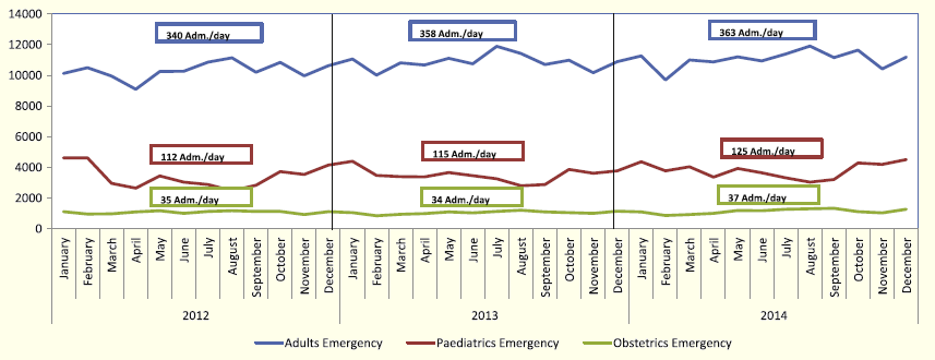
Fig­ure 1: Admis­sions to the Gen­eral, Pedi­atric and Obstet­ric Emer­gency (2012–2014), at Braga Hos­pi­tal

From the sever­ity point of view, based on the Man­ches­ter Triage [GPT 2018], 65% of Braga Hos­pi­tal admis­sions are either very urgent or urgent, but there is a slight increase in 2013 and 2014, com­par­ing to 2012, of admis­sions due to mat­ters of lit­tle urgency (green line) as can be seen in Fig­ure 2.

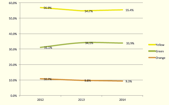
Fig­ure 2: Pro­por­tional Dis­tri­b­u­tion of Sever­ity Lev­els through the Man­ches­ter Triage (2012–2014), at Braga Hos­pi­tal

The arrival of patients to the hos­pi­tal can be done in two ways: either elec­tive, an activ­ity pro­grammed days or weeks in advance, or emerg­ing, when a patient arrives at the ED in an unplanned man­ner. This arrival can be for rea­sons asso­ci­ated with epi­demi­o­log­i­cal fac­tors (aging pop­u­la­tion, chronic­ity of dis­eases), envi­ron­men­tal fac­tors (cold or heat weather peaks), eco­nom­i­cal fac­tors (eco­nomic cri­sis, cir­cum­ven­tion on pay­ment of user fees, a decreas­ing use of pri­vate ser­vices) or social fac­tors (sys­tem­atic recourse to emer­gency ser­vices on cer­tain days of the week and hours of the day). Stud­ies show that the turnout to the ED is not a ran­dom process [Abra­ham et al. 2009; Cham­pion et al. 2007] and very often peaks in demand are related with sea­son­al­ity of patholo­gies, to pub­lic or school hol­i­days, or to the time of day or day of the week. The occu­pa­tion of hos­pi­tal beds is bro­ken down between elec­tive admis­sions, planned in advance, and admis­sions through the ED (about 56% of the total hos­pi­tal­iza­tions). It is accepted as good prac­tice that patients are admit­ted within 6 h from arrival at the ED (about 9% of the total patients that come through the ED). The afflu­ence of patients through the ED raises the level of uncer­tainty for the need of beds to a point that fre­quently same-day sur­gi­cal activ­i­ties have to be can­celed and the typol­ogy of oper­a­tive plans have to be changed, favor­ing out­pa­tient surg­eries instead of sur­gi­cal patients due to beds unavail­abil­ity. As there are fund­ing restric­tions, a bal­ance between cost and effec­tive­ness must be obtained in resources allo­ca­tion. The abil­ity to pre­dict the vol­ume of demand in the ED would, in the short term, enable the cor­rect allo­ca­tion of clin­i­cal teams for emer­gency ser­vice assur­ing suit­able wait­ing times for care, and adjust­ing the avail­abil­ity of beds in the hos­pi­tal for the appro­pri­ate response to the influx of severe and urgent clin­i­cal pic­tures.

3. Methods

3.1 Definitions

We con­sider arrivals all episodes in which the patient goes through the admin­is­tra­tive reg­is­tra­tion process, regard­less of when he leaves. Upon arrival to the ED, the patient is exam­ined by a nurse in the triage process, and is headed for a med­ical spe­cial­ist to start the diag­no­sis and han­dling of com­plaints. The expec­ta­tion is that his stay in the hos­pi­tal will be less than 24 h, except in more com­plex sit­u­a­tions that require a more pro­longed clin­i­cal approach, in which case he will be for­warded to the inpa­tient admis­sion. The rea­sons for a patient to be dis­qual­i­fied with­out com­plet­ing the process are: when the patient is treated and sent back home with indi­ca­tions of con­ti­nu­ity addressed to the fam­ily doc­tor/spe­cial­ist in out­pa­tient reg­i­men pro­grammed; trans­ferred to another hos­pi­tal, when the clin­i­cal sit­u­a­tion is sta­bi­lized and the patient should return to the hos­pi­tal source, in his area of res­i­dence; ref­er­enced for intern­ment in the hos­pi­tal; and, very rarely, when the patient is deceased dur­ing the episode. All episodes of aban­don­ment, after hav­ing been admin­is­tra­tively reg­is­tered, account to the met­ric of arrivals to the urgency.

3.2 Study Design

From Jan­u­ary 2012 there is reli­able data for arrivals to the ED of the Braga Hos­pi­tal. This infor­ma­tion includes the patient’s name, age, gen­der, date and time of arrival, triage sort­ing, des­ti­na­tion after triage, date and time of release, and release jus­ti­fi­ca­tion. The first phase of this work con­sisted in the col­lec­tion and pro­cess­ing of the data. The pre­dic­tive model will work on data col­lected from Jan­u­ary 2012 to Decem­ber 2013 (test period), with 177,769 arrivals on 2012 and 185,132 arrivals on 2013; the results thus obtained will be com­pared to the data from 2014 (eval­u­a­tion period), in order to deter­mine the accu­racy of the esti­mates obtained by pre­dic­tion of the num­ber of arrivals.

4. Statistical Experiments

The vari­able under study is the arrival of users to the ED. The data from 2012 and 2013, more than 350,000 records, was treated and sta­tis­ti­cal tests were per­formed. All sta­tis­ti­cal analy­sis were per­formed using IBM SPSS v21 [Field 2013] and Excel 2010 [Burns and Bush 2007].

Users’ arrival to the ED was ana­lyzed regard­ing the month of the year, the day of the week and the time of the day. To give an idea about the mag­ni­tude of the data, Fig­ure 3 shows the day-aver­age arrivals dis­tri­bu­tion per month (a), per week day (b) and along the day (c) (con­sid­er­ing data from Jan­u­ary 2012 to Decem­ber 2013). This fig­ure shows that the great­est demand is in Feb­ru­ary (533.7 arrivals per day), on Mon­day (567.6 arrivals per day) and dur­ing the day there are two peaks for increased demand which are at the start of the morn­ing and early after­noon.

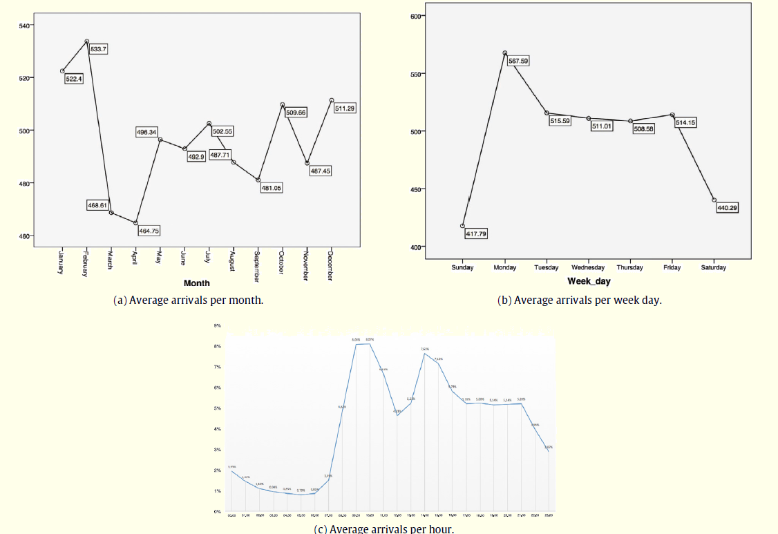
Fig­ure 3: Aver­age Num­ber of Arrivals (Jan­u­ary 2012–Decem­ber 2013)

The daily arrivals dis­tri­bu­tion dur­ing the test period, Fig­ure 4, presents an almost per­fect nor­mal dis­tri­bu­tion.

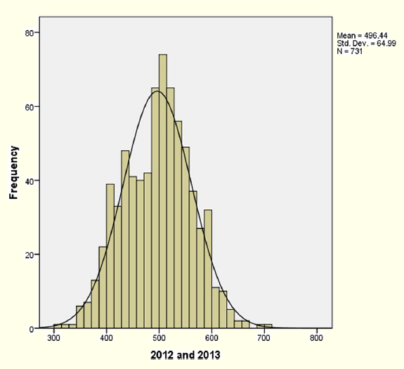
Fig­ure 4: Arrivals Dis­tri­b­u­tion dur­ing the Test Period (2012–2013)

4.1 Correlation Tests

Some authors [Diaz et al. 2001; Kam et al. 2010; Linares and Jaz 2008] sug­gest that max­i­mal, min­i­mum, mean tem­per­a­ture and humid­ity are the envi­ron­men­tal vari­ables that can influ­ence the ED arrivals. Jones and Joy [2002] also use tem­per­a­ture and pre­cip­i­ta­tion. Mar­cilio et al. [2013], McCarthy et al. [2008] and War­gon et al. [2010] refer that using pre­cip­i­ta­tion this gives some uncer­tainty to the model giv­ing also almost no improve­ments to the pre­ci­sion on the fore­cast. As stated in [Mar­cilio et al. 2013] one of the motives for dif­fer­ent opin­ions on intro­duc­ing or not the tem­per­a­ture on the fore­cast mod­els are the fact that the dif­fer­ent stud­ies occur in dif­fer­ent geo­graph­i­cal areas with the ED show­ing dif­fer­ent char­ac­ter­is­tics as well.

In this work sev­eral envi­ron­men­tal vari­ables were stud­ied in order to iden­tify their rela­tion to the ED arrivals. Those that showed greater cor­re­la­tion were the pre­cip­i­ta­tion and the max­i­mum tem­per­a­ture but even these were not sig­nif­i­cant in rela­tion to the cor­re­la­tion of the arrivals.

The Pear­son bivari­ate Cor­re­la­tion test in SPSS pro­duces a coef­fi­cient r that quan­ti­fies the strength and direc­tion of the rela­tion between two vari­ables. The Pear­son cor­re­la­tion also assesses the pres­ence of sta­tis­ti­cal evi­dence of a lin­ear rela­tion­ship between the same time series, rep­re­sented by the ρ value. The Pear­son test was used to study the cor­re­la­tion between the arrivals to the ED and the envi­ron­men­tal vari­ables pre­cip­i­ta­tion and max­i­mum tem­per­a­ture whose data is from Under­ground [2001]. Regard­ing pre­cip­i­ta­tion and arrivals, the result was r(ρ) = −0.102(0.006). This cor­re­la­tion coef­fi­cient char­ac­ter­izes a weak neg­a­tive lin­ear rela­tion­ship between the vari­ables, i.e., arrivals decrease with an increased level of pre­cip­i­ta­tion. Regard­ing arrivals and max­i­mum tem­per­a­ture there is no cor­re­la­tion, accord­ing to the result r(ρ) = −0.028(0.457). The same tests were made for the hol­i­days, and the results obtained r(ρ) = −0.188(p) with p < 0.01, con­cludes for the exis­tence of a
weak cor­re­la­tion.

4.2 Autocorrelation Test

Auto­cor­re­la­tion is the self lin­ear depen­dence of a vari­able in sep­a­rate moments. It is a sta­tis­ti­cal mea­sure that indi­cates the rela­tion between val­ues of the same vari­able sep­a­rated in time. For exam­ple, the auto­cor­re­la­tion of period 1 mea­sures the ratio between con­sec­u­tive val­ues of the vari­able while the auto­cor­re­la­tion of period 12 indi­cates the rela­tion­ship between val­ues sep­a­rated by 12 peri­ods of time. These tests mea­sure the degree of asso­ci­a­tion between two obser­va­tions, Y_t and Y_t−k, when the effects of the peri­ods prior to k(1, 2, 3, . . . , k − 1), are elim­i­nated.

The tests showed a strong cor­re­la­tion on 7 days’ time series of arrivals. A par­tial auto­cor­re­la­tion was iden­ti­fied, height­en­ing the cor­re­la­tion between each 7 days period, with even greater empha­sis on adja­cent days (Fig­ure 5). The results obtained in the auto­cor­re­la­tion tests will be a deter­min­ing fac­tor for the con­struc­tion and improve­ment of the pre­dic­tion model to imple­ment.

5. Forecasting Methods

Sta­tis­ti­cal tests hav­ing been car­ried out, the next step would be the def­i­n­i­tion of a fore­cast­ing model for the num­ber of arrivals to the ED. There are sev­eral types of mod­els, such as the Mov­ing Aver­age, the Expo­nen­tial Smooth­ing, the Holt-Win­ters, the ARIMA, among oth­ers. These mod­els have been used in areas such as Finance, Sta­tis­tics, Eco­nom­ics, Oper­a­tions Research, Indus­try and Health [War­gon et al. 2010].

Sev­eral types of fore­cast mod­els were tested, and final choice was for ARIMA type mod­els (Auto Regres­sive-Inte­grated-Moving Aver­age) [Gerolimetto 2010], so these will be fur­ther explained. ARIMA mod­els pro­vide an approach to time series and fore­cast­ing and are one the most widely-used method­olo­gies to time series fore­cast­ing, pro­vid­ing com­ple­men­tary approaches to the prob­lem. ARIMA mod­els aim to describe the auto­cor­re­la­tions in the data and use the fol­low­ing
nota­tion:

ARIMA(p, d, q)

where p is the order of the autore­gres­sion process (AR), d is the degree of dif­fer­en­ti­a­tion involved (I) and q is the order of the Mov­ing Aver­age process (MA). To make the time series sta­tion­ary (trend removal), it is pre­vi­ously made d dif­fer­ences between the data. The math­e­mat­i­cal expres­sion for this kind of mod­els
is:

Yt = φ₁Y_t−1 + φ₂Y_t−2 + ... + φ_pY_t−p + e_t − θ₁e_t−1 − θ₂e_t−2 − ... − θ_qe_t−q

where Yt is the vari­able value at time t, φ and θ are the model para­me­ters for the autore­gres­sive and mov­ing aver­age terms, respec­tively, and et are the resid­ual term rep­re­sent­ing ran­dom dis­tur­bances that can­not be pre­dicted [Makri­dakis 1989]. Although there is no limit to the vari­ety of ARIMA mod­els, in prac­tice it is sel­dom nec­es­sary to use val­ues of p, d and q above 2. It is worth not­ing that only three val­ues 0, 1 or 2, to the para­me­ters p, d and q, are suf­fi­cient to rep­re­sent the wide range of time series, from the most diverse con­texts.

ARIMA mod­els are also capa­ble of mod­el­ing a wide range of sea­sonal data. The sea­sonal ARIMA model is formed by includ­ing addi­tional sea­sonal para­me­ters and is writ­ten as fol­lows:

ARIMA(p, d, q)(P, D, Q)^s

where P, D and Q rep­re­sent the same as p, d and q for the sea­sonal part of the model, and s is the num­ber of peri­ods in a sea­sonal cycle.

These mod­els have the fol­low­ing char­ac­ter­is­tics: the­o­ret­i­cally they are suit­able for most data series; they are able to model vari­a­tions, trends, autore­gres­sive­ness and sea­son­ally mov­ing aver­age; an uni­vari­ate approach method, it requires no exter­nal data; also, the sta­tis­ti­cal soft­ware is widely avail­able.

5.1 Accuracy Measurements

In this study, accu­racy was used as the main cri­te­rion for select­ing a fore­cast­ing method, and our assess­ment of fore­cast accu­racy is based on the Mean Absolute Per­cent­age Error (MAPE) met­ric:

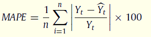
where Y_t and Ŷ_t are the real arrivals and the fore­casted arrivals in time t, respec­tively and n is the num­ber of time units. This mea­sure was used to eval­u­ate and com­pare the per­for­mance of the stud­ied mod­els in the test period. An inde­pen­dent scale sta­tis­tic as the MAPE enables the direct com­par­i­son of a model fore­cast over mul­ti­ple time series.

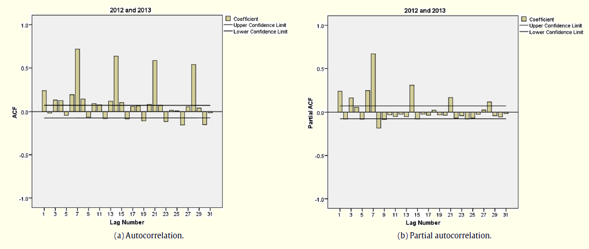
Fig­ure 5: Auto­cor­re­la­tion Test

6. Results

Exper­i­ments were made with var­i­ous types of mod­els using Ora­cle Crys­tal Ball soft­ware [Gen­try 2008] and Fore­cast Pro V 3.0 [Delur­gio 2005]. In the Table 1 are the MAPE val­ues for some of these mod­els, using test period arrivals (2012–2013).

Table 1: MAPE Val­ues for Six Mod­els

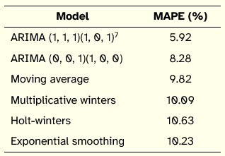
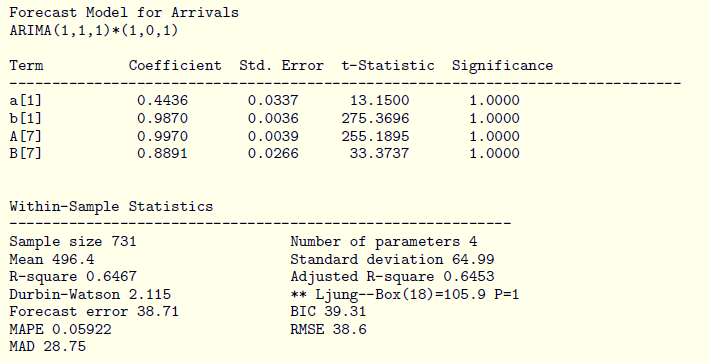
The best model for the test period was the ARIMA (1, 1, 1) (1, 0, 1)⁷ with MAPE = 5.92%:

Y_t = 0.4436Y_t−1 − 0.9870e_t−1 + 0.9970Y_t−7 −0.8891e_t−7 + e_t (2)

fol­lowed by ARIMA (0, 0, 1)(1, 0, 0) with MAPE = 8.28%:

As already iden­ti­fied in the auto­cor­re­la­tion test, the s value, num­ber of peri­ods in a sea­sonal cycle, is 7 days. The report pro­vided by the soft­ware Fore­cast Pro for ARIMA (1, 1, 1)(1, 0, 1)⁷ model (2) is:

Using the ARIMA (1, 1, 1)(1, 0, 1)⁷ model (2), the fore­cast for the eval­u­a­tion period (2014), gives MAPE= 6.34%. The fact that the arrivals for 2014 is actual data, allows to eval­u­ate the per­for­mance level of the fore­cast model.

Fig­ure 6 dis­plays the monthly val­ues of MAPE for 2014. As shown, there are 4 months with a lower than 5% MAPE fore­cast. The increase in the error through­out the year denotes pos­si­ble rel­e­vance to obtain short-term esti­mates, tak­ing into account the vari­abil­ity influx of ED, which is inde­pen­dent of sea­son­al­ity.

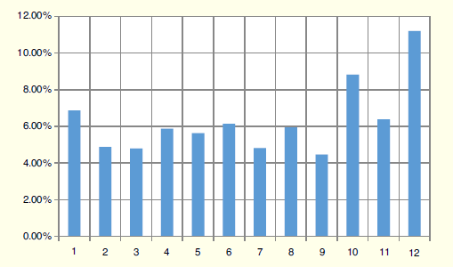
Fig­ure 6: Monthly MAPE Val­ues Fore­cast for 2014

Fig­ure 7 shows the model behav­ior to esti­mate Jan­u­ary 2014, the month fol­low­ing the series of data that sup­ports it. Fore­cast­ing the arrivals for the sec­ond, third and fourth weeks of Jan­u­ary 2014, this time includ­ing the data from the first week of 2014 in addi­tion to the data from the test period, we obtain bet­ter results (dot­ted line in Fig­ure 8). The model was ‘‘fed’’ with the val­ues of the week imme­di­ately pre­ced­ing the fore­casted period. Over the next 3 weeks, the model already adjusted its behav­ior based on the knowl­edge of the first week data. In this sit­u­a­tion MAPE = 5.22% for the first four weeks of Jan­u­ary 2014 against MAPE = 6.84%. This is a very impor­tant achieve­ment of this work. Con­sid­er­ing the MAPE val­ues only for the sec­ond week, we obtain MAPE = 5.72% against MAPE = 9.29%.

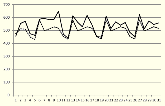
Fig­ure 7: Fore­casted Val­ues (dashed line) vs. Actual Data (solid line) for Jan­u­ary 2014

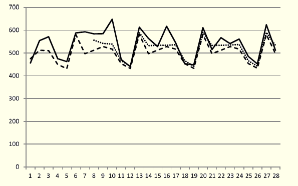
Fig­ure 8: Fore­casted Val­ues (dashed line, dot­ted line) vs. Actual Data for the Last Three Weeks of Jan­u­ary 2014

Aim­ing to only pre­dict arrivals next week the model behaves with very good per­for­mance. This obser­va­tion shows that the knowl­edge of the pre­vi­ous week’s arrivals is very impor­tant for a more accu­rate fore­cast.

7. Conclusions

Due to the high com­plex­ity of resources asso­ci­ated with the oper­a­tion of the ED, the impor­tance of fore­cast­ing mod­els of arrivals is absolutely crit­i­cal for resource plan­ning in the hos­pi­tal. The obtained model allows pre­dic­tions for a week or a month with a very good qual­ity level. Accu­rate fore­cast­ing of ED arrivals decreases the can­cel­la­tions of planned admis­sions and opti­mizes
the beds allo­ca­tion to the real demand. The human resources allo­ca­tion is also adjusted accord­ing to the needs of beds and the num­ber of work sta­tions to patient care in the ED, with the aim of pro­vid­ing uni­ver­sal access to health­care.

Acknowledgments

This work was sup­ported by The Por­tuguese Foun­da­tion for Sci­ence and Tech­nol­ogy (FCT) by the ALGO­RITMI R&D Cen­ter and project PEST-OE/EEI/UI0319/2014. The authors are very grate­ful to the Hos­pi­tal de Braga—Escala Braga, Sociedade Gestora do Esta­b­elec­i­mento, S.A., for pro­vid­ing the data.

References

• Abra­ham, G., G. B. Byrnes and C. A. Bain (2009). Short-term fore­cast­ing of emer­gency inpa­tient flow. IEEE Trans­ac­tions on Infor­ma­tion Tech­nol­ogy in Bio­med­i­cine 13(3), 380–388.

  Bern­stein, S. L., D. Aron­sky, R. Duseja, S. Epstein, D. Han­del, U. Hwang, M. McCarthy, K. J. McConnell, J. M. Pines, N. Rath­lev, R. Schafer­meyer, F. Zwe­mer, M. Schull and B.R. Asplin (2009). The effect of emer­gency depart­ment crowd­ing on clin­i­cally ori­ented out­comes, soci­ety for aca­d­e­mic emer­gency med­i­cine, emer­gency depart­ment crowd­ing task force. Aca­d­e­mic Emer­gency Med­i­cine 16(1), 1–10.

  Billings, J., T. Georghiou, I. Blunt and M. Bard­s­ley (2013). Choos­ing a model to pre­dict hos­pi­tal admis­sion: An obser­va­tional study of new vari­ants of pre­dic­tive mod­els for case find­ing. BMJ Open 3(8)..

  Boyle, J., M. Jes­sup, J. Crilly, D. Green, J. Lind, M. Wal­lis and G. Fitzger­ald (2010). Pre­dict­ing emer­gency depart­ment admis­sions. Emer­gency Med­i­cine Jour­nal 29(5), 358–365.

  Burns, A, C. and R. F. Bush (2007). Basic Mar­ket­ing Research using Microsoft Excel Data Analy­sis. Upper Sadle River, New Jer­sey: Pren­tice Hall Press.

  CRRNEU (2012). Reavali­ação da Rede Nacional de Emergên­cia e Urgên­cia. Comis­são de Reavali­ação da Rede Nacional de Emergên­cia/Urgên­cia

  Cham­pion, R., L. D. Kins­man, G. Lee, K. Mas­man, E. May, T. M. Mills and R. J. Williams (2007). Fore­cast­ing emer­gency depart­ment pre­sen­ta­tions. Aus­tralian Health Review 31(1), 83–90.

  Delur­gio, S. (2015). Guide to Fore­cast Pro from Win­dows. http://fore­cast.umkc.edu

  Diaz, J., J. C. Alberdi, M. S. Pajares, C. Lopez, R. Lopez, M. B. Lage and A. Otero (2001). A model for fore­cast­ing emer­gency hos­pi­tal admis­sions: effect of envi­ron­men­tal vari­ables. Jour­nal of Envi­ron­men­tal Health 64(3), 9–15.

  Field, A. (2013). Dis­cov­er­ing Sta­tis­tics Using IBM SPSS Sta­tis­tics, 4^th edi­tion. Lon­don, Eng­land: SAGE Pub­li­ca­tions.

  Gen­try, B., D. Blank­in­ship and E. Wain­wright (2008). Crys­tal Ball User Man­ual 11.1. Ora­cle.

  Gerolimetto, M. (2010). ARIMA and SARIMA Mod­els. http://www.dst.unive.it/margherita/TSLec­ture­Notes6.pdf

  GPT (2018). Sis­tema de Triagem de Man­ches­ter. Grupo Por­tu­gus de Triagem. http://www. grupopor­tugues­triagem.pt

  Hoot, N. R. and D. Aron­sky (2008). Sys­tem­atic review of emer­gency depart­ment crowd­ing: Causes, effects, and solu­tions. Annals of Emer­gency Med­i­cine 52(2), 126–136.

  Hoot, N. R., C. Zhou, I. Jones and D. Aron­sky (2007). Mea­sur­ing and fore­cast­ing emer­gency depart­ment crowd­ing in real time. Annals of Emer­gency Med­i­cine 49(6), 747–755.

  Hoot, N. R., S. K. Epstein, T. L. Allen, S. S. Jones, K. M. Baum­lin, N. Chawla and D. Aron­sky (2009). Fore­cast­ing emer­gency depart­ment crowd­ing: An exter­nal, mul­ti­cen­ter eval­u­a­tion. Annals of Emer­gency Med­i­cine 54(4), 514–522.

  Jones, S. A. and M. P. Joy (2002). Fore­cast­ing demand of emer­gency care. Health Care Man­age­ment Sci­ence 5(4), 297–305.

  Kam, H. J., J. O. Sung and R. W. Park (2010). Pre­dic­tion of daily patient num­bers for a regional emer­gency med­ical cen­ter using time series analy­sis. Health­care Infor­mat­ics Research 16(3), 158–165.

  Linares, C. and J. Daz (2008). Impact of high tem­per­a­tures on hos­pi­tal admis­sions: Com­par­a­tive analy­sis with pre­vi­ous stud­ies about mor­tal­ity (Madrid). Euro­pean Jour­nal of Pub­lic Health 18(3), 317–322.

  Makri­dakis, S. and S. C. Wheel­wright (1989). Fore­cast­ing Meth­ods for Man­age­ment, fifth edi­tion. New York: John Wiley & Sons.

  Mar­cilio, I., S. Hajat and N. Gou­veia (2013). Fore­cast­ing daily emer­gency depart­ment vis­its using cal­en­dar vari­ables and ambi­ent tem­per­a­ture read­ings. Aca­d­e­mic Emer­gency Med­i­cine 20(8), 769–777.

  McCarthy, M. K., S. L. Zeger, R. Ding, D. Aron­sky, N. R. Hoot and G. D. Kelen (2008). The chal­lenge of pre­dict­ing demand for emer­gency depart­ment ser­vices. Aca­d­e­mic Emer­gency Med­i­cine 15(4), 337–346.

  Under­ground, C. W. (2001). Weather under­ground. http://por­tuguese.wun­der­ground.com

  War­gon, M., E. Casalino and B. Guidet (2010). From model to fore­cast­ing: a mul­ti­cen­ter study in emer­gency depart­ment. Aca­d­e­mic Emer­gency Med­i­cine 17(9), 970–978.

  Wiler, J.L, R. T. Grif­fey and T. Olsen (2011). Review of mod­el­ing approaches for emer­gency depart­ment patient flow and crowd­ing research. Aca­d­e­mic Emer­gency Med­i­cine 18(12), 1371–1379.